|
This is part three of a series of
technical articles on the aerodynamics of control-line flying. It appeared in the
December 1967 edition of American modeler. Figures, equations, and graphs do not
begin at #1 because this is a continuation of the series. I do not yet have the
edition for part 2. Here is
Part 1.
The Academy of Model Aeronautics is granted tax-exempt status because part of its
charter is for activity as an educational organization. I think as time goes on, it gets
harder for the AMA for fulfill that part of its mission because presenting anything even
vaguely resembling mathematics or science to kids (or to most adults for that matter),
is the kiss of death for gaining or retaining interest. This article, "Control-Line Aerodynamics
Made Painless," was printed in the December 1967 edition of American Modeler, when graphs,
charts, and equations were not eschewed by modelers. It is awesome. On rare occasions
a similar type article will appear nowadays in Model Aviation for topics like
basic aerodynamics and battery / motor parameters. Nowadays, it seems, the most rigorous
classroom material that the AMA can manage to slip into schools is a box of gliders and
a PowerPoint presentation. That and a few scholarships each year keep the tax status
safe... for now.
Control-Line Aerodynamics Made Painless
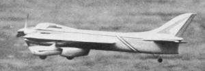 In a dead-stick glide, Dave Gierke's excellently
designed NOVI (October issue) displays its smooth, flowing lines.
 Altitude angle measurement instrument
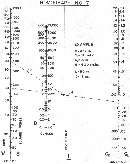
 Nomograph No. 7
Your airplane is smarter than you are! It knows and obeys every aerodynamics law.'
Which is to say that "old devil" math is really a useful tool. By its careful application
many 'mysterious' factors are made plain.
By Bill Netzeband
Editor's Note: In the Sept./Oct. and Nov./Dec., 1966 issues were presented Parts I
and II of this series. Both the editor and author lacked faith at that time that enough
control-liners would seriously consider the mathematical aspects of design. Many favorable
letters have been received since. Some called us "chicken" for quitting, This filial
article now is published with the observation that it should have been printed long ago.
Reviewing the introduction to this informa-tive series we may have supplied rather
shaky reasons for going to all these lengths to properly design a "rock on a string."
The fact that most published designs were "brute force" (cut-fit-crash) developed didn't
always detract from their final shape.
It has become apparent that anyone, no matter how misinformed, can run down the rest
of us who "roll our own" designs. So let us elevate the purpose of these reports thusly:
Your finished airplane is smarter than you are! It instinctively knows every solitary
aerodynamic law, and unquestioningly obeys them to the letter. It therefore behooves
us to learn as many of the important laws as possible so that we don't demand something
which that smart lil' ole' airplane cannot do.
We will deal mostly in how and how much with flights into why, where it is important.
Mathematics are an essential part of our process, since without numbers, the principles
are pretty academic and often misleading. As promised, the derivations of equations generally
won't be detailed, except where the final product is clarified. It is also planned to
suggest test methods and/or devices, so that ultimately we may communicate on the firm
base of measured performance, rather than "Gee Whiz, it sure looked good." So much for
reintroduction.
Since you've already peeked at the sketches, we're dealing with the major lateral
and vertical force diagram to evaluate surface lift requirements, maximum level flight
altitudes and a method for measuring the maximum lift for an airplane. Also a discussion
of the propeller as a gyroscope with perhaps the answer to some of your "mysterious"
crashes.
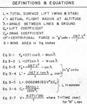
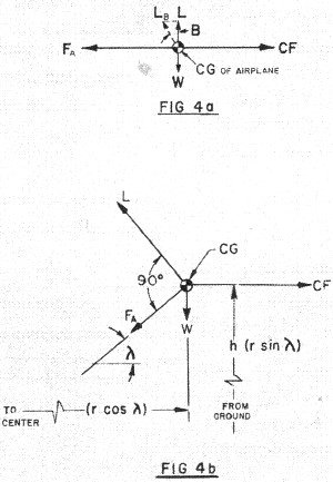
Fig. 4a illustrates the major physical forces generated by restraining a mass (our
CG) in horizontal flight level with the handle. CF is centrifugal force from Part 1,
Nomograph No.3. FA is line tension equal and opposite to CF. W & L are airplane weight
and the surface lift necessary to just equal W. This is the simplest case, since each
vector system is essentially "in line." This is the flight mode used to determine maximum
line tension and trim lift.
It should be noted here that wing lift is assumed to be normal (perpendicular) to
the chord line. If the airplane is banked into the circle (vector LB), the wing must
generate more life to support W, but will allow FA to decrease. For small angles, up
to 10 degrees LB is almost equal to L, and the reduction of FA is W tan B, since L=W.
For a heavy ship (3 lb.) at a 10-degree bank angle, line tension would be reduced almost
0.5 lb. without requiring additional lift. This effect is directly opposite if banked
outward, and is not proportional to airspeed.
The use of this phenomenon is not desirable for aerobatics or combat, but could be
used for in Navy Carrier (outbank) or a heavy Rat or Speed job (bank in). The most reliable
method to obtain this force is to place the line(s) guide above (bank in) or below (outbank)
the CG of the airplane. Any other method to generate a roll force (wing warping, ailerons,
weight, etc.) will add detrimental side effects (no pun intended) such as added drag,
an angle proportional to airspeed or adverse yawing effects.
It can be readily shown that a bank angle exists for any line length and air-speed
which would give zero line tension (W tan B = CF). Actually, the amount of weight is
not a factor, since CF can be reduced to its equivalent "g" factor by factoring out W.
Therefore bank angle for zero line tension becomes a product of line length and airspeed.
For 60' lines at 100 mph, angle B would be 85°51' (11 g's) NOT too practical, but interesting.
It is entirely possible that the wing cannot generate the lift necessary to do a kooky
trick like that, anyway.
Points against banking in, are the land-ing and takeoff, where "g" factors of less
than 1/2 are generated. Control can be lost, and/or the airplane could "come in" on you.
Meanwhile, back to important stuff. Fig. 4b represents the real meat of this sandwich.
CF is now calculated for a radius less than the line length (r cos λ). λ is the angle
of elevation, which is some-what easier to visualize than actual altitude (h), and is
more convertible for varying line lengths. (sin λ= h/r). Under the conditions of 4b,
FA is less than FA for horizontal flight (Fig. 4a) since the lift vector (L) now assumes
some horizontal restraining forces. L will be shown to become tremendous at high angles,
and maximum lift capability of an airplane will limit the maximum elevation angle.
Perhaps we should point out that we are dealing with level flight, not to be confused
with looping and such maneuvers. It is not so difficult to prove that an airplane can
be zoomed into lift factors not available in level sustained flight due to kinetic energy
stored in the system.
Equations 3-1 and 3-2 were derived by conventional vector analysis and are the basis
for the rest of our juggling. To simplify trial analysis we factored out weight (W),
reducing the force system to "g" units, now dependent only on airspeed (V) elevation
angle (A) and line length (r). We then substituted the equation for CF in terms of "g"
units, arriving at equa-tions 3-3 and 3-4. By specifying (V), and (r), we can calculate
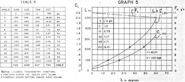
line tension and lift at various elevation angles. Calculations are reduced by use of
Nomograph No. 3 (July/Aug.
'66) and Trigonometric Functions annotated in Table 4. Simple results are plotted
on Graph 5 for an airplane on 60' lines traveling at a constant 100 mph. To get actual
forces, simply multiply "g" factors by W. Sample numbers would apply to a slow Rat at
26 ounces. L in "g"s are listed.
Come now the engineering compromises. We cannot get lift without drag. Increased lift
causes increased drag. so without being able to increase thrust, the higher we fly. the
slower we go. O.K.? Since high flying is one large bone of contention in contest judging,
we should know where a "point of diminishing returns" is reached. Or should I fly at
the maximum allowed height or not? (We do not advocate cheating!) Space does not allow
complete evaluation of induced drag at this sitting. so complete analysis of actual speed
reduc-tion versus "apparent speed increase" will merely be dangled before you. right
now. ("Apparent speed" is equal to V actual/cos λ).
Of immediate interest is maximum lift. since we now have most of the machinery to
measure it. To evaluate a given airplane a graph or series of point calculations leading
to L versus λ are necessary. For most CL airplanes a Lift Coefficient (CL)
of 0.9 is about the limit before going into hard stall conditions. Nomograph 7 will calculate
L, D, or CL and CD depending on the order of procedure. (Eq. 3-5
and 3-6) If. as we have right now, values for L, we can calculate CL. The
example shown on the face of the Nomograph can be solved for CL by proceeding
as follows: 1) Pick up wing area (S) and lift required (L) with straight edge and hold
crossing point 1; 2) Holding 1, swing to V on left hand scale, reading answer CL
on RH scale.
Lift coefficient (CL) is a figure of merit defining the lift per unit area
of a wing for specific conditions of Reynolds Number and angle of attack. It is necessary
to introduce it, unadorned, so that we have common ground to complete this discus-sion.
As we said, except for a high efficiency stunt wing with high lift devices, most CL
wings will stall at CL = 0.9. At this point drag is extremely high, and lift
will decrease if you force the wing to higher angles of attack. An end point for high
lift without excessive decrease in airspeed due to induced drag is closer to 0.3 or 0.4.
Having plotted or tabled L and corresponding CL versus λ, pick out the
CL of interest, and note the elevation angle. This is the maximum angle at
which you can fly level (if CL were 0.9) or maybe the highest to fly for best
"apparent speed."
During all of this, a detailed study of FA indicates a small decrease in line tension
as λ increases. From Eq. 3-1, at 90 degrees line tension disappears except for airplane
weight coming down. From Eq. 3-3 it appears to be different, that line tension in "g"
units is equal to horizontal g's reduced by sin λ (which varies from 0 to 1.0). The apparent
mathematical anomaly is caused by the fact that under practical circumstances CF for
a zero radius is infinite, such that correct procedures require definition of max-min
values by calculus. We cannot practically reach these limits, so they are hereby ignored.
If we apply wing areas of 90 sq. in. and 140 sq. in. to our sample plot and a fixed
weight of 26 ounces, we have a country fair argument for the larger area Rat Racers.
F'rinstance, applying CL of 0.4 for best speed at altitude, the 90 comes in at 15 degrees,
the 140 at 26. Maximum elevation for the 90 is conservatively 35 degrees as opposed to
49 degrees for the big one. Granted you can zoom maybe ten degrees higher to pass, but
you won't stay up there long! Note also, that line tension is reduced by only 0.9 "g"
even at 60 degrees, although the speed reduction we know exists will cause an actual
reduction. since CF will decrease. Finally, 20' (max. racing altitude, except passing)
represents an λ, of 19.5 degrees. not too encouraging for the 90. if the 140's decide
to run at 20 ft!
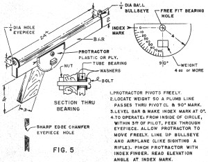
If we had a way to measure V and (λ) while flying our airplane, without wind, at its
highest altitude, we could calculate its maximum lift coefficient. Luckily, both can
be measured with reasonable accuracy, if you want to take a little time to build a crude
theodolite from Fig. 5. Using the gadget like a pistol, sighting through the eyepiece
until the bulls eye covers the airplane, while several laps are clocked with a stop watch,
you have both angle and velocity nailed down. (V) can be calcu-lated from Eq 3-7.
Knowing the angle (λ) and velocity, we can plug these numbers, along with (r), into
equation 3-4 and come up with (L') in g's. By multiplying (L') by (W), we have (L max)
from which CL max can be calculated from Nomograph 7 (Eq. 3-5 or 3-6). This
would settle many questions, like in stunt as to just what CL is a prac-tical
maximum. The reduction in airspeed from level flight (minimum drag) will give a measure
of drag increase. It is needless to tell you that this information is useless, unless
you dig in and apply it, isn't it?
Particularly significant in stunt and combat is maximum lift, since this determines
the minimum looping radius. It has become apparent that indiscriminant use of full-size
airfoil data has led to some extremely optimistic turn radii. We seldom achieve the efficiency
of a large wing at high speed. Therefore, to derive useful data we are using experimental
measurements such as this one to write our own book.
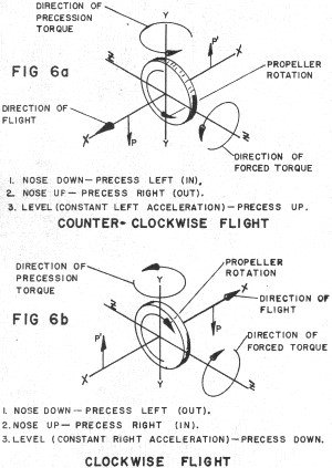
The next phenomenon has been pub-lished before, without specifically pointing out
one dangerous area. The propeller acts as a gyroscope since it is a rotating mass and
numerical analysis proves that under adverse conditions it can generate enough precession
torque to cause trouble. Referring to Fig. 6a we see the conventional forces associated
with a gyro. The physics of the system are too complex to put down here; only the results
will be presented. Essentially what occurs for conventional prop rotation (CCW when viewed
from front), when the rotation axis X-X (prop shaft) is tilted, a reaction torque appears
in one of the axes perpendicular to the X-X axis.
In the case shown in Fig. 6a, we are flying in the conventional direction (CCW) and
move the nose down (coupling forces P-P'). This rotation is about the Z-Z axis and the
precession torque appears about the vertical axis Y-Y in the direction shown. All of
the forces involved here are couples (two equal and opposite forces in the same plane,
but not along the same line). A couple is handled as a torque (a force on an arm causing
rotation) and can be balanced only with an equal and opposite couple or torque. These
facts cause the precession force to be independent of its distance from the CG, so long
or short nose lengths do not affect it. Therefore, the illustrated torque appears at
the CG turning the nose into the circle.
As noted, nose up turns produce nose out torque, while the steady left hand acceleration
of level flight produces a small nose up torque. These are all real, sport fans. The
amount of precession torque depends directly on the mass (weight) of the propeller, its
diameter (specifically the CG location of each blade), the engine rpm and the angular
acceleration (rate of airplane turning) which is in turn dependent on airspeed and turn
radius. The larger any of these, except turn radius, the larger the precession torque.
There are several danger points in the precision aerobatic pattern, where high rates
of nose-down pitch are required, the square eight and the middle two corners of the hourglass.
Noting. the reversal of conditions in inverted flight (Fig. 6b) one can include the second
and third reverse wingover corners and bottoms of outside square loops. The effect can
vary from momentary loss of control to complete loss of airplane.
In the early days with the climb and dive maneuvers we had troubles, too. To deliberately
look for this force John Barr and I took his late "Lil Satan" with ST 15 diesel power,
increased the stabilator area for sharper turns and performed hairy climbs with sharp
pullouts. Finally with a 9-3 prop, relatively slow airspeed (low line tension) and high
rpm, we started getting it every time. The nose would swing in violently, the ship would
completely slack off and float to the other side. During the initial test series we were
ready and could regain control before it crashed, but during a night session she pulled
the bit so quickly and accidentally that the end arrived. The stunt ship with its marginal
centrifugal force and a combat rig with a slight warp and high rpm mill are prime victims
for this force. Since plastic props weigh about 50 percent more than wood props they
will generate 50 percent more precession force.
The effect of the small nose-up or down-precession in level flight explains the apparent
stability increase while flying inverted since the effect is destabilizing in CCW flight
and stabilizing in CW. This probably explains why the majority of the "developed" stunt
rigs end up with a raised thrust line, to partially compensate for the precession effect
on trim.
Posted February 27, 2011
|